Regression: Introduction
Regression
We are going to explain the behavior of $y$ with $x$ with a linear model
\begin{equation}
y = \beta_0 + \beta_1 x + u
\label{e:regression}
\end{equation}
where $x$ and $y$ are the vectors of the data, and the vector $u$ represents the other factors that affect $y$.
If the other factors remain constant, than the changes in $y$ are fully
explained by the changes in $x$:
$$
\Delta y = \beta_1 \Delta x.
$$
Indeed, let $(x_1, y_1, u_1)$ and $(x_2, y_2, u_2)$ are two tripples
of the data such that $u_1 = u_2 = u$, i.e., $\Delta u = 0$.
Equation (\ref{e:regression}) is applied twice:
\begin{gather*}
y_1 = \beta_0 + \beta_1 x_1 + u
\\
y_2 = \beta_0 + \beta_1 x_2 + u
\end{gather*}
Subtracting equations we get
$$
\Delta y = \beta_1 \Delta x
\quad\quad \mathrm{if } \Delta u = 0.
$$
Example
We regress wage on the years of education: \begin{equation} wage = \beta_0 + \beta_1 educ + u \label{e:wage:regr} \end{equation} Then $\beta_1$ measures the change in hourly wage given another year of education, holding all other factors fixed. Some of those factors include labor force experience, innate ability, tenure with current employer, work ethic, and numerous other things.
Assumptions on $u$
$u$ is $0$ on average
Mathematically, it means that
\begin{equation}
\mathbf{E} u = 0.
\label{e:zeromean}
\end{equation}
This assumption is not restrictive because the intercept $\beta_0$ represents a vertical shift.
The crucial (and restrictive) assumption states that
$x$ and $u$ do not correlate. It means that
the expected value of $u$ given $x$ does not depend on $x$:
\begin{equation}
\mathbf{E}(u|x) = \mathbf{E}u.
\label{e:meanindependenceonx}
\end{equation}
Combining \eqref{e:zeromean} and \eqref{e:meanindependenceonx}, we end up with a single equation
\begin{equation}
\mathbf{E}(u|x) = \mathbf{E}u = 0
\label{e:zerocondmean}
\end{equation}
- In real problems, $u$ is typically unobserved.
- The absence of the correlation is always something to discuss
Example (model):
The score at the final exam linearly depends on the classes attended and unobserved factors (such as ability):
$$ score = \beta_0 + \beta_1 attend + u. $$Discuss whether assumption \eqref{e:zerocondmean} holds.
Linear dependence of the expected mean of $y$ on $x$
Takig the model equation \eqref{e:regression} and using assumption \eqref{e:zerocondmean}, compute the conditional expectation of $y$ given $x$:
\begin{equation} \mathbf{E}(y | x) = \beta_0 + \beta_1 x. \end{equation}For any value of $x$, there is the population of the dependent variable $y | x$. The mean of the population belongs to the line $y' = \beta_0 + \beta_1 x$.
- $y$ consists of systematic part $\mathbf{E}(y | x)$
- and unsystematic part $u$
Derivation of $\beta_0$ and $\beta_1$
- independence of $u$ and $x$ in formal terms: transformation of \eqref{e:zerocondmean}:
- sample $(x_i, y_i)$, $i = 1, 2, \ldots, n$
- compute the covariance of the both hand side of the regression
with $x$: $$ \mathbf{Cov}(x,y) = \beta_1 \mathbf{Cov}(x,x), $$ $$ \rho_{xy}\sigma_x\sigma_y = \beta_1 \sigma_x^2, $$ where $\rho_{xy}$ is the coefficient of the correlation between $x$ and $y$, $\sigma_x$ and $\sigma_y$ are the standard deviations. Then \begin{equation} \beta_1 = \rho_{xy}\cdot\frac{\sigma_y}{\sigma_x}. \label{e:beta1p} \end{equation}
substitute sample for random variable characteristics in assumptions \begin{equation} \hat{\beta}_1 = \frac{\sum_{i=1}^n (x_i - \bar{x})(y_i - \bar{y})} {\sum_{i=1}^n (x_i - \bar{x})^2} \label{e:beta1mod} \end{equation}
Another possibility to use sample characteristics: substitution into the assumptions from the very beginning
or \begin{gather} \mathbf{E}(y - \beta_0 - \beta_1 x) = 0 \\ \mathbf{E}(x(y - \beta_0 - \beta_1 x)) = 0 \end{gather}
- after the substitution: \begin{gather} \frac{1}{n}\sum_{i=1}^n (y_i - \beta_0 - \beta_1 x_i) = 0 \\ \frac{1}{n}\sum_{i=1}^n x_i(y_i - \beta_0 - \beta_1 x_i) = 0 \end{gather}
The solution:
\begin{gather} \hat{\beta}_1 = \frac{\sum_{i=1}^n (x_i - \bar{x})(y_i - \bar{y})} {\sum_{i=1}^n (x_i - \bar{x})^2} \label{e:beta1alt} \\ \hat{\beta}_0 = \bar{y} - \hat{\beta}_1 \bar{x} \label{e:beta0} \end{gather}
Alternatively, one may write \begin{equation} \hat{\beta}_1 = \hat{\rho}_{xy} \cdot \left(\frac{\hat{\sigma}_y}{\hat{\sigma}_x}\right) \label{e:beta1mod2} \end{equation}
You see that \eqref{e:beta1mod2} coincides with \eqref{e:beta1mod}.
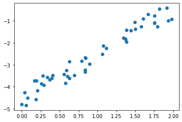
import numpy as np
from numpy import random
import matplotlib.pyplot as plt
from sklearn.linear_model import LinearRegression
import scipy.stats
rng = np.random.RandomState(1)
nn = 50
#Generate nn = 50 normal random values and save them in x
x = 2 * rng.rand(nn)
# y[] is defined as a linear function of x[] up to a random factor
y = 2 * x - 5 + rng.rand(nn)
#plot the dependence of y on x
plt.scatter(x, y);
Construction of the best fit
- we use the above mathematics
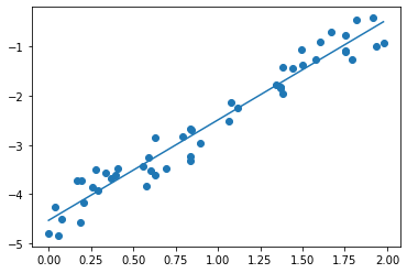
beta1 = scipy.stats.pearsonr(x, y)[0] * np.std(y) / np.std(x)
beta0 = np.mean(y) - beta1 * np.mean(x)
xx = np.linspace(np.min(x), np.max(x))
yy = beta0 + beta1 * xx
plt.scatter(x, y)
plt.plot(xx, yy)
beta0, beta1
Residiuals:
$$ u_i = y_i - \hat{y}_i = y_i - \hat{\beta}_0 - \hat{\beta}_1 x_i $$We can formulate the problem:
what are the numbers $\beta_0$ and $\beta_1$ that minimize
$$
\sum_i (y_i - \beta_0 - \beta_1 x_i)^2
$$
Prove that
- these $\beta_0$ and $\beta_1$ are the values defined above
- the sum of residuals is zero: $$ \sum_i u_i = 0 $$ hint: recall that $\mathbf{E}u = 0$
- Other possiblities to define residuals
Goodness-of-fit
- total sum of squares SST $$ \mathrm{SST} = \sum_{i=1}^n (y_i - \bar{y})^2 $$
- the explained sum of squares $$ \mathrm{SSE} = \sum_{i=1}^n (\hat{y}_i - \bar{y})^2 $$
the residual sum of squares $$ \mathrm{SSR} = \sum_{i=1}^n \hat{u}_i^2 $$
Property: SST = SSE + SSR
- $$ R^2 = \mathrm{SSE}/\mathrm{SST} = 1 - \mathrm{SSR}/\mathrm{SST} $$
- $R^2$ signals the quality of the fit. Lesser values of $R^2$ suggest that the quality is questionable
sst = np.sum((y - np.mean(y))**2)
haty = beta0 + beta1 * x
sse = np.sum((haty - np.mean(y))**2)
u = y - haty
ssr = np.sum(u**2)
print(sst, sse, ssr, sst-sse-ssr)
To think
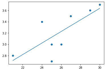
the Wooldridge handbook, pages 77-78 of the file, questions 1-4
Comment to question 3:
# type
import numpy as np
y = np.array([2.8, 3.4, 3.0, 3.5, 3.6, 3.0, 2.7, 3.7])
x = np.array([21, 24, 26, 27, 29, 25, 25, 30])
print(np.round(beta0, 2), np.round(beta1, 3))
Expected value and variance of the estimate
We place the proof only for $\hat{\beta}_1$
$\newcommand{\Exp}{\mathbf{E}}$ $\newcommand{\Var}{\mathbf{Var}}$
Indeed, we have already proved: $$ \hat{\beta}_1 = \frac{\sum_{i=1}^n (x_i - \bar{x})y_i}{\sum_{i=1}^n (x_i - \bar{x})^2} $$ Substituting $y_i = \beta_0 + \beta_1 x_i + u_i$ and opening brackets, we get \eqref{e:regr:beta1}.
Warning: We compute the mathematical expectation with respect to $\mathrm{u}$, given the sample $\mathrm{x}$. That is why all terms $x_i-\bar{x}$ and the denominator are constants, whereas the expected value of each $u_i$ is zero, $\Exp u_i=0$
As a result, the second term in the right hand side of (\ref{e:regr:beta1}) disappears, and the estimate is unbiased
$\newcommand{\Var}{\mathbf{Var}}$
The variances of the random term conditional on $x$ does not depend on $i$: $$ \Var(u_i \,|\, x) = \sigma^2 $$
$\newcommand{\Exp}{\mathbf{E}}$ $\newcommand{\Var}{\mathbf{Var}}$
Recall that the computation is performed under assumption that the sample is fixed (but $u$ is random). Then $$ \Var(\hat{\beta}_1) = \frac{1}{\Sigma_{xx}^2} \sum_{i=1}^n (x_i - \bar{x})\Var(u_i) = \frac{1}{\Sigma_{xx}^2} \Sigma_{xx} \sigma^2 = \frac{\sigma^2}{\Sigma_{xx}} $$
In practice, the variance of the estimator is not known. A natural estimate of the variance appears when the variance $\sigma^2$ of the errors is estimated with the data. Let $\hat{s}^2$ be this estimate. Then we introduce the estimator $\big(S(\hat{\beta}_1)\big)^2$ for variance of $\hat{\beta}_1$ as $$ \big(S(\hat{\beta}_1)\big)^2 = \frac{\hat{s}^2}{\Sigma_{xx}}, $$
$\newcommand{\Prob}[1]{\mathsf{P}\{#1\}}$
Testing
- Alternative hypothesis: $\beta_1 > 0$
- Significance level: $\alpha = 5\%$
- Rule: compute $t$-statistics $$ t_{\hat{\beta}_1} = \frac{\hat{\beta}_1} {S(\hat{\beta}_1)} $$ if the probability $\Prob{X > t_{\hat{\beta}_1}} < \alpha$, i.~e., the $t$-statistics is so large that larger values are extremely rare (with respect to the chosen significance level), reject the null hypothesis.
- The inequality in probabilities is equivalent to the fact that the $t$-statistics is larger than the $\alpha$-quantile: $$ t_{\hat{\beta}_j} > q_{\alpha, n-2}, $$ where the quantile can be found in the corresponding table (taking into account the number of freedom $n-2$)
#the above example example (several slides ago)
#$H_1$ is two-sided
from scipy.stats import chi2
import numpy as np
y_hat = [beta0 + beta1*x_cur for x_cur in x]
u_hat = [y[i] - y_hat[i] for i in range(len(y))]
u_hat_std = np.std(u_hat)
t_statistics = beta1/u_hat_std
df = len(y)-2w
tmp = chi2.cdf(t_statistics, df)
if tmp < 0.5:
    pvalue = 2*tmp
else:
    pvalue = 2*(1-tmp)
print('statistics = {:.3f}'.format(t_statistics), 'p-value = ', '{:e}'.format(pvalue),
      'df = {:.2f}'.format(df))
alph = [0.005, 0.01]
for a in alph:
    if tmp < 0.5:
        print('significance level = ', a, '; lower cut-off = {:.3f}'.format(chi2.ppf(a/2, df)),
          '; chi-2 < cut-off', t_statistics < chi2.ppf(a/2, df))
    else:
        print('significance level = ', a, '; upper cut-off = {:.3f}'.format(chi2.ppf(1-a/2, df)),
          '; chi-2 > cut-off', t_statistics > chi2.ppf(1-a/2, df))
Instrumental variables: Example
- How does amount of time spent studying affect exam scores?
- How does a certain drug affect blood pressure?
- How does stress affect heart rate?
In general: we want to understand whether or not some predictor variable affects a response variable
Problem: Other factors can affect both predictor and response variable
However, other variables like time spent exercising, overall diet, and stress levels also affect blood pressure
Thus, if we run a simple linear regression using the drug as our predictor variable and blood pressure as our response variable, we cannot be sure that the regression coefficients will accurately capture the effect that the drug has on blood pressure because outside factors (exercise, diet, stress, etc.) could also be playing a role
An instrumental variable is a third variable introduced into the regression analysis that is correlated with the predictor variable, but uncorrelated with the response variable. By using this variable, it becomes possible to estimate the true causal effect that some predictor variable has on a response variable
Introduce a new variable in our example: Proximity to pharmacy
- Proximity to pharmacy likely correlates with the fact that an individual take the drug
- but almost certainly does not correlate with the blood pressure
- Stage 1: Fit a regression model using the instrumental variable as the predictor variable $$ \mathtt{certain\ drug} = \beta_{0} + \beta_{1}\mathtt{proximity} $$
The outcome of the first stage is the predicted values $\hat{d} = (\hat{d}_1,\ldots, \hat{d}_n)$ of the $\mathtt{certain\ drug}$
- Stage 2: regress the blood pressure on the predicted values of the $\mathtt{certain\ drug}$
$$
\mathtt{bp} = b_0 + b_1\hat{d}
$$
- Test ${b}_1 \ne 0$ against ${b}_1 = 0$ in a standard way
- It is highly correlated with the predictor variable.
- It is not correlated with the response variable.
- It is not correlated with the other variables that are left out of the model (e.g. proximity is not correlated with exercise, diet, or stress)
Summary
- The best linear fit as the regression resulted from economics assumptions
- Construction of the best linear fit
- Mean and variance of the estimate of the regression coefficient $\beta_1$
- Hypothesis testing: $\beta_1 \ne 0$
- Instrumental variables
This is the end of the course


