Goodness of the fit and Pearson test
Numerical example and theoretical background
- $5$ events are observed, whereas the background event rate is $\nu_b = 0.5$
- Are a new type of events observed?
$n_{\text{obs}} = 5$ $$ \mathsf{Prob}\{ n \ge n_{\text{obs}} \} = 1-\sum_{n=0}^{n_{\text{obs}}-1} f(n;0,\nu_b) = 1 - \sum_{n=0}^{n_{\text{obs}}-1} \frac{\nu_b^n}{n!}e^{-\nu_b} $$
import numpy as np
def prob_greater_poisson(n, p):
    #<n> is the number of observed events
    #<p> is the mean value of the Poisson distribution
    s = 0
    power_cur = 1
    factorial_cur = 1
    exp_val = np.exp(-p)
    for i in range(n):
        s += power_cur / factorial_cur * exp_val
        power_cur *= p
        factorial_cur *= i + 1
    return 1-s
ss = prob_greater_poisson(5, 0.5)
print('Probability to observe these or more extreme data, p-value:', ss)
Possible interpretation of the above computation:
the probability to get 5 or more events is equal to $1.7 \cdot 10^{-4}$ under the hypothesis that they are generated by the background process
more detailed investigation: plus-minus interval
- the variance of the Poisson random variable, $\sigma^2=\mathbf{Var}X = \mathbf{E}X$
- our estimate of $\nu = 5$, $\nu = \nu_s + \nu_b$
- adding $\sigma$ as the plus/minus component, we get $\hat{\nu} = 5 \pm \sqrt{5}$
- the same for the specific event rate: $\hat{\nu}_s = 4.5 \pm 2.3$
the interval $\hat{\nu}_s = 4.5 \pm 4.6$ with doubled plus-minus component includes $0$, which is misleading as we recall the $p$-value equaled to $1.7\cdot 10^{-4}$
* The interval estimate invloves the probabilities that the Poisson random variable with the mean $\nu=5$ fluctuates downward to $\nu_b = 0.5$ or lower. That is incorrect * On the contrary, `p-value` indicates that the Poisson random variable with mean $\mu_b = 0.5$ fluctuates to $n_{\text{obs}} = 5$ or higher- Question:
How to resolve this controversion between the arguments based on the p-value and the interval estimate?
- The practice of displaying measured values of Poisson variables with an error bar given by the square root of the observed value unfortunately encourages the incorrect interpretation
Errors in the parameter estimations
- Assume that the background rate is $0.8$ instead of $0.5$. Then the
p-valueis
ss = prob_greater_poisson(5, 0.8)
print('Probability to observe these or more extreme data, p-value:', ss)
print('New_probability / Old_probability = ',
      prob_greater_poisson(5, 0.8) / prob_greater_poisson(5, 0.5))
- Thus, the new probability is approximately $10$ times larger
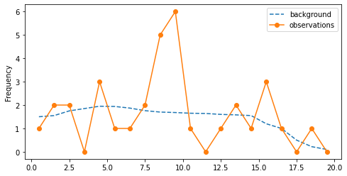
Deviation of the binned data from the background
x_back = [i+0.5 for i in range(20)]
v_back = [1.50, 1.55, 1.75, 1.85, 1.95, 1.94, 1.87, 1.76, 1.70, 1.68, 1.65, 1.64, 1.60, 1.58,
         1.55, 1.20, 1.0, 0.50, 0.22, 0.10]
x_obs = [i+0.5 for i in range(20)]
v_obs = [1, 2, 2, 0, 3, 1, 1, 2, 5, 6, 1, 0, 1, 2, 1, 3, 1, 0, 1, 0]
import matplotlib.pyplot as plt

fig = plt.figure(figsize=(8, 4))
ax = plt.subplot(1,1,1)
ax.plot(x_back, v_back, label='background', linestyle='--')
ax.plot(x_obs, v_obs, label='observations', marker='o', markersize=6)
ax.set_ylabel('Frequency')
ax.legend()
plt.show()
Outliers
- Are values $n(8.5) = 5$ and $n(9.5) = 6$ outliers that are incosistent with the background level?
print('Background rate when the observed values seem to be extreme',
      v_back[8] + v_back[9])
Attempt to use the previous approach
- To what extent $5+6=11$ events are extreme when the background rate is $3.38$
- The above formula for the
p-valuereturns
print('Probability {n >= 11 | rate = 3.38} = ', prob_greater_poisson(11, 3.38))
- What is the conclusion? Outliers?
Drawback
- The place of the peak is chosen aposteriori. The computed probability is related to the peak at the specific placed chosen after the experiment is conducted. It does not take into account that the other data in a better agreement with the background
Pearson's $\chi^2$ test
- Statistics: $\displaystyle\chi^2 = \sum_{i=1}^N \frac{(n_i - \nu_i)^2}{\nu_i}$
If the data $\mathbf{n} = (n_1,\ldots,n_N)$ are Poisson distributed with mean values $\mathbf{\nu} = (\nu_1,\ldots,\nu_N)$ and the number of entries in each bin is not too small then - the statistics $\chi^2$ follows the $\chi^2$ distribution with $N$ degrees of freedom. This holds regardless of the distribution of the variable $\mathbf{x}$
- larger $\chi^2$ corresponds to a larger discrepancy between data and the hypothesis
- In our example,
#p[] is a background process; n[] corresponds to observations
def chisquare_simple(n, p):
    if len(n) != len(p) or len(n) == 0 or n == None or p == None:
        return None
    chisquare = 0
    for i in range(len(n)):
        chisquare += (n[i] - p[i])**2 / p[i]
    return chisquare
print(chisquare_simple(v_obs, v_back))
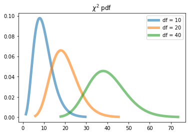
Visualizing $\chi^2$ distribution
https://docs.scipy.org/doc/scipy/reference/generated/scipy.stats.chi2.html
from scipy.stats import chi2
import numpy as np
import matplotlib.pyplot as plt
fig, ax = plt.subplots(1, 1)
dfs = [10, 20, 40] #degree of freedom
for df in dfs:
    x = np.linspace(chi2.ppf(0.001, df), chi2.ppf(0.999, df), 1000)
    ax.plot(x, chi2.pdf(x, df), '-', lw=5, alpha=0.6, label=f'df = {df}')
plt.title('$\chi^2$ pdf')
plt.legend()
plt.show()
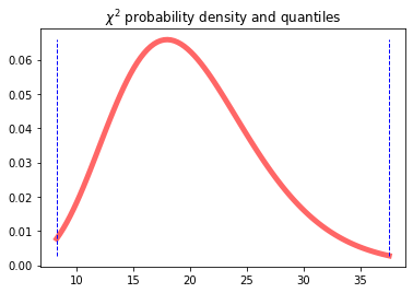
Returning to our example
df = len(v_obs)
chi2.ppf(0.01, df), chi2.ppf(0.99, df) #print quantiles
fig, ax = plt.subplots(1, 1)
dfr = 20 #degree of freedom
x = np.linspace(chi2.ppf(0.01, dfr), chi2.ppf(0.99, dfr), 100)
ax.plot(x, chi2.pdf(x, dfr), 'r-', lw=5, alpha=0.6, label='chi2 pdf')
level = 0.01
quantile1 = chi2.ppf(level, dfr)
quantile2 = chi2.ppf(1-level, dfr)
ax.plot([quantile1, quantile1], [min(chi2.pdf(x, dfr)), max(chi2.pdf(x, dfr))], 'b--', lw=1)
ax.plot([quantile2, quantile2], [min(chi2.pdf(x, dfr)), max(chi2.pdf(x, dfr))], 'b--', lw=1)
ax.set_title('$\\chi^2$ probability density and quantiles')
plt.show()
df = len(v_obs)
alph = [0.001, 0.005, 0.01]
stat = chisquare_simple(v_obs, v_back)
print('statistics', stat)
for a in alph:
    print('significance level = ', a, '; cut-off = ', chi2.ppf(1-a, df), '; chi-2 > cut-off',
         stat > chi2.ppf(1-a, df))
Question:
Can we reject the hypothesis that just the background process is observed?
* No, at the chosen significance levels
Question:
What a p-value does correspond to our observations
* Type 1-chi2.cdf(stat, df)
1-chi2.cdf(stat, df)
More real assumptions
- We assumed that each $n_i$ is a Poisson random variable and the sum $n_{\text{tot}} = \sum_{i=1}^N n_i$ is itself a Poisson variable with a predicted mean value $\nu_{\text{tot}} = \sum_{i=1}^N \nu_i$
- New set of assumptions: $n_{\text{tot}}$ is fixed (from observations), $n_i$ is multinomial distributed with $p_i = \nu_i / n_{\text{tot}}$.
- Then statistics: $\displaystyle\chi^2 = \sum_{i=1}^N \frac{(n_i - p_i n_{\text{tot}})^2}{p_i n_{\text{tot}}}$
- As a result, the statistics $\chi^2$ is still asymptotically $\chi^2$ distributed but the number of degrees of freedom is $N-1$
- Nothing changed in the statistics in our example.
- The degree of freedom is reduced by one
- Standard computation (corresponding to $N-1$ degree of freedom) is repeated below
import numpy as np
from scipy.stats import chi2
df_mod = len(v_obs) - 1
alph = [0.001, 0.005, 0.01, 0.1]
stat = chisquare_simple(v_obs, v_back)
print('statistics = ', stat, 'p-value = ', '{:.3f}'.format(1-chi2.cdf(stat, df_mod)))
for a in alph:
    print('significance level = ', a, '; cut-off = {:.3f}'.format(chi2.ppf(1-a, df_mod)), '; chi-2 > cut-off',
         stat > chi2.ppf(1-a, df_mod))
print(df_mod)
Drawback: Small number of values in the bins
We must refuse the theoretical distribution and construct the distribution with the Monte-Carlo method.
The following code computes $N = 1000$ samples with the $\chi^2$ statistics and order the array of statistics
from scipy.stats import poisson
N = 1000 #number of repetition in the Monte-Carlo simulations
stat_mc = []
for _ in range(N):
    v_mc = [poisson.rvs(v) for v in v_back]
    stat_mc.append(chisquare_simple(v_mc, v_back))

stat_mc = sorted(stat_mc)
import bisect
alph = [0.001, 0.005, 0.01, 0.1] #must be between 0 and 1
stat = chisquare_simple(v_obs, v_back)
print('statistics = ', stat, 'p-value = {:.3f}'.format(1-bisect.bisect_left(stat_mc, stat) / len(stat_mc)))
for a in alph:
    cutoff = stat_mc[int(round((1-a)*N))]
    print('significance level = ', a, '; cut-off = {:.3f}'.format(cutoff), '; statistics > cut-off', stat > cutoff)
We observe an increase of $p$-value from $0.056$ to $0.104$


