Bootstrap (pulling up the hair)
 |
 |
Generation of random numbers with given distribution
Some theory
$\newcommand{\Prob}[1]{\mathsf{P}\{#1\}}$
- $X$ is a random variable with the cumulative distribution function $F(x)$:
$$
F(x) = \Prob{X \le x}
$$
TheoremIf $F$ is continuous function then the random variable $F(X)$ is uniformly distributed on $[0,1]$Proof:
Question:
Where is the continuity used?
* We solved the equation $F(x) = t$ for any $t \in [0, 1]$
$\newcommand{\rv}[1]{\mathbf{#1}}$
Corollary
Let $\rv{R}_n - (\rv{r}_1, \ldots, \rv{r}_n)$ be the vector of independent random variables that are uniformly distributed over $[0, 1]$. Let also $F(x)$ be a continuous function, and there is a vector $\rv{Z}_n = (\rv{z}_1,\ldots,\rv{z}_n)$ such that
$$
\rv{r}_i = F(\rv{z}_i).
$$
Then each component of the vector $\rv{Z} = (\rv{z}_1,\ldots,\rv{z}_n)$ is distributed with the cumulative distribution function $F$.
Classical distributions
- Easy usage of libraries
- Advanced: Metropolis–Hastings algorithm
Example
$$
F(x) = 1-e^{-ax},
\quad
\rv{Z}_n = -\frac{1}{a}\log(1-\rv{R}_n)
$$
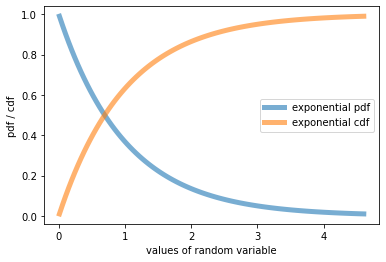
With classical distributions, you can use standard library functions as in the following example with the exponential distribution. Populate your cell with the following code
import numpy as np
from scipy.stats import expon #import exponential distribution
import matplotlib.pyplot as plt
fig, ax = plt.subplots(1, 1)
#<name>.ppf(alpha) returns alpha-quantile
x = np.linspace(expon.ppf(0.01), expon.ppf(0.99), 100)
#<name>.pdf(x) returns the value of the probability distribution function
ax.plot(x, expon.pdf(x), lw=5, alpha=0.6, label='exponential pdf') #graph of pdf
ax.plot(x, expon.cdf(x), lw=5, alpha=0.6, label='exponential cdf') #graph of ddf
ax.set_xlabel('values of random variable')
ax.set_ylabel('pdf / cdf')
ax.legend()
plt.show()
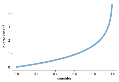
#one can display the inverse cdf with <name>.ppf() method
fig, ax = plt.subplots(1, 1)
x = np.linspace(0, 1, 100)
ax.plot(x, expon.ppf(x), lw=5, alpha=0.6, label='exponential inverse pdf') #graph of pdf^{-1}
ax.set_xlabel('quantiles')
ax.set_ylabel(r'inverse cdf $F^{-1}$')
plt.show()
Question:
What will you see in the graph if add values being closer to $0$ and $1$ to the definition of $x$ changing, f.e.,
x = np.linspace(0, 1, 100)
to
x = np.linspace(0, 1, 1000)
* The graphs will follow a significant growth at the right (why?); the changes at the left are minor
* Make these changes and observe the difference
Manual computation of inverse pdf
Function $F(x)$ is absent in the library
- Frequently used technique (even in this manual)
- If $F^{-1}$ is not defined rigorously, its approximation is of interest
- Let $[m, M]$ be such an extent interval that it definitely contains possible observations
- Define a detailed uniform bins on $[m, M]$:where $N$ is large
bin = np.linspace(m, M, N)
import numpy as np
m = 0
M = 1
N = 1000
vals_avail = np.linspace(m, M, num=N)
vals_avail[:10], vals_avail[-5:-1]
- The number $N$ must be much larger in practical computation
- The value is constrained by the power of the computer
- Compute and save values of the (direct) cdf at the chosen points
- We will follow this program with a distribution defined in the educational purpose below
def cdf_str(x):
    return 0.5 * (x + np.sqrt(x))
z_avail = [cdf_str(v) for v in vals_avail]
np.transpose(z_avail[:5]), np.transpose(z_avail[-5:-1])
#Inverse pdf
from scipy.interpolate import interp1d
import random
import matplotlib.pyplot as plt
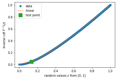
ppf_str = interp1d(z_avail, vals_avail, kind='linear')
v_new = np.linspace(m, M, num=17)
fig, ax = plt.subplots(1, 1)
ax.plot(z_avail, vals_avail, 'o', cdf_str(v_new), v_new, '--')
random.seed(1)
v_tmp = random.random()
ax.plot(v_tmp, ppf_str(v_tmp), 's', markersize=12)
ax.legend(['data', 'linear', 'test point'], loc='best')
ax.set_xlabel('random values $z$ from $[0, 1]$')
ax.set_ylabel('inverse cdf $F^{-1}(z)$')
plt.show()
Combing previous code with graph with two functions
- specifying cdf
- assumed that the argument of cdf is np.array()
- otherwise include
x = np.array(x)into the code
- defining inverse cdf
import numpy as np
from scipy.interpolate import interp1d
def cdf_complex(x):
    return 0.5 * (x + np.sqrt(x))
def ppf_appr(m=0, M=1, N=1000):
    vals_avail = np.linspace(m, M, num=N)
    z_avail = [cdf_complex(v) for v in vals_avail]
    ppf = interp1d(vals_avail, z_avail, kind='linear')
    return ppf
Hypothesis testing based on empirical distribution function with unknown paramters
- $x_1 < x_2 < \ldots < x_n$ is ordered sample of independent observations of the random variable with the distribution function $F(x;\theta)$, where $\theta$ is a parameter
- Hypothesis $H_0$: the sample agrees with this distribution with some unknown value of the paramter at a specified signicance level
Idea of the solution
- Estimate $\theta$ as some $\hat{\theta}$
- If the expected value is a parameter, compute the mean.
- In general case, the likelihood estimate is used (will be discussed next week)
- Construct the KS-statistics $$ D = n^{1/2}\max|F(x;\hat{\theta}) - \hat{F}_n(x)| $$ where $\hat{F}_n$ is the empirical distribution function
- Compare the statistics with the corresponding $\alpha$-quantile; $\alpha$ is the significance level
Drawback of the above method
- this method corresponds to the case when no unknown parameters are involved and the agreement with a pre-defined distribution is estimated
- the existence of the parameter alters the situation
- the distance $D$ becomes less than that following the Kolmogorov-Smirnov distribution
Question:
If one still uses the quantiles from the KS distribution, how it affects the probability of the type I error (reject $H_0$ when it is correct)?
* The distances are smaller than they should be* The rejection of $H_0$ is more rare
* The rule corresponds a significance level that is larger then given significance level
* The probability of the type I error is larger than expected
- What is a possible improvement of the solution?
Improvement: multiple estimates of the parameter
- Estimate model parameter many times, say $N = 1000$ or more
- In the case of the unknown expected value, one can choose $N$ times half of the sample
- and choose the mean of this sub-sample as the estimate of the expected value
- For any estimate $\hat{\theta}$ of the parameter $\theta$, (
ivaries from0toN-1)- create $n$ values $v = (v_1, \ldots, v_n)$ from the theoretical distribution with the estimated value of the parameter ($n$ is the sample size)
- find the KS-statistics, i.e., the KS-distance $D_i$ between the empirical distribution function built on $v$ and the theoretical distribution function $F(x;\hat{\theta})$
- Order the computed distances $D_i$
- As a result, $i/N$-quantiles are obtained, where $i=0,\ldots,N-1$
Bootstrap
History and purpose
- Bradly Efron, 1977
- Create empirical distribution, provided the sample
- Using the created empirical distribution as theoretical one, generate pseudo-samples of an arbitrary size
- The unknown parameters and their distributions are estimated with the pseudo-samples
- The basic example is the estimate of the variance for any statistics
Bootstrap from a discrete sample
- $\mathbf{x} = (x_1, \ldots, x_n)$ is a given random sample from an unknown distribution $\rv{X}$
- Task: estimate parameters of $\rv{X}$
- Solution
- generate $N$ times:
for i in range(N): - sample $\mathbf{y}^{(i)} = (y_1, \ldots, y_n)$ from $\mathbf{x}$ performing choice with replacement:
- result: vectors $\mathbf{y}^{(1)}$, $\ldots$, $\mathbf{y}^{(N)}$
- generate $N$ times:
#Example of the sampling with replacement
import random
random.seed(1)
x_example = [0, 2.5, 2022, 1, 0]
sample_new = random.choices(x_example, k=15)
sample_new
Question:
Why is number $0$ most frequent?
* It appears twice in the initial sample
#EStimate of the variance
import numpy as np
def bootstrap_var(x, N=100, seed=1):
    random.seed(seed)
    variances = []
    for i in range(N):
        sample_new = random.choices(x, k=len(x))
        variances.append(np.var(sample_new))
    return variances
variances = bootstrap_var([0, 2.5, 2022, 1, 0])
np.mean(variances), np.var(x_example)
- all obtained estimates are conditional to the observation of the initial vector $\mathbf{x} = (x_1, \ldots, x_n)$
- these conditional estimates tend to the true estimates as $n \to \infty$
- typically, bootstrap estimate is located below a real variance
Bootstrap with continuous distribution function
Motivation
- The true distribution can be continuous, but the bootstrapped distribution is discrete
- This can be improved through the approximation of the observed discrete distribution by a continuous function
Linear approximation
- Notation
- $\mathbf{x} = (x_1, \ldots, x_n)$ is an observed vector
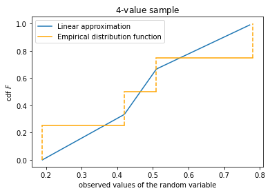
- empirical distribution function $F_{\text{edf}}$ consists of steps with $$ F_{\text{edf}}(x) = i / N, \quad x_i < x \le x_{i+1} $$ we re-order the coordinates and keep the old notation: $x_1 < \ldots < x_n$; the probability of $x_i = x_{i+1}$ is $0$ for continuous distributions, but this case is easily included into the construction: e.g., if $x_{i-1} < x_{i} = x_{i+1} < x_{i+2}$, then $F_{\text{edf}}(x_i) = (i-1)/N$ and $F_{\text{edf}}(x_{i+1}+0) = (i+1) / N$
- Approximation
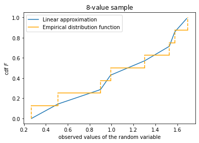
- Place a point at the vertical gap of each $F_{\text{edf}}(x)$ jump
- Connect these points (e.g., with
numpy.percentile()# Syntax of numpy.percentile() numpy.percentile(arr, percentile, axis=None, out=None, overwrite_input=False, keepdims=False)
arr - array_like, this is the input array or object that can be converted to an array.
percentile – array_like of float Percentile or sequence of percentiles to compute, which must be between 0 and 100 inclusive
Choice of the points on the vertical gaps
- There are infinitely many possibilities
numpy.percentilechooses the lowest point at the left gap, the highest point at the right gap and goes from bottom to the top uniformly in-between
Question:
If the sample contains from $5$ points, what are the locations of the delimiters of the vertical gaps?
* Ratios: from left to right: $0$, $0.25$, $0.5$, $0.75$, $1$
The second example is below
#technical: plots empirical distribution (step-like function)
def plt_empirical_dstr(x, clr=None, label='Empirical distribution function'):
    frac_before = [i / len(x) for i in range(len(x))]
    frac_after = [(i+1) / len(x) for i in range(len(x))]
    for i in range(len(x)):
        plt.plot([x[i], x[i]], [frac_before[i], frac_after[i]], linestyle='--',
                color=clr_perc)
        if i == 0 and clr != None:
            plt.plot([x[i], x[i+1]], [frac_after[i], frac_after[i]], label=label)
        elif i < len(x)-1 and clr != None:
            plt.plot([x[i], x[i+1]], [frac_after[i], frac_after[i]])
        elif i == 0:
            plt.plot([x[i], x[i+1]], [frac_after[i], frac_after[i]], label=label)
        elif i < len(x)-1:
            plt.plot([x[i], x[i+1]], [frac_after[i], frac_after[i]])
#empirical distribution and linear approximation to it with N = 8 points
import numpy as np
import random
import matplotlib.pyplot as plt
random.seed(1)

N = 8
x = []
for _ in range(N):
    x.append(random.uniform(0, 2))
x = np.array(sorted(x))

num_percentiles = 100
t = []
val = []
for uni in range(num_percentiles):
    t.append(uni / num_percentiles)
    val.append(np.percentile(x, uni))

fig, ax = plt.subplots(1, 1)
ax.plot(val, t, label='Linear approximation')
plt_empirical_dstr(x, clr='orange')
ax.legend()
ax.set_xlabel('observed values of the random variable')
ax.set_ylabel('cdf $F$')
ax.set_title('${:d}$-value sample'.format(N))
plt.show()
Practical computation
- Compute the bootstrapped sample $z$
u = [100*random.random() for _ in range(len(x))]
z = np.percentile(x, u)
- The empirical distribution of the vector $z$ approximates the empirical distribution of the (first observed) vector $x$
- Use the vector $z$ to estimate the paramter
- Compute the mean of the estimates
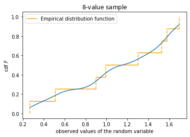
Kernel method
Definition of a specific kernel,
which is, clearly, non-unique.
For any $z \in \mathbb{R}$ we put
$$
F_{\text{kernel}}(z) = \frac{1}{n}
\sum_{i=1}^n \Phi\left(\frac{z-x_i}{s}\right)
$$
where $n$ is the number of observations and $\Phi$ is cdf of the standard normal distribution, and $s$ is a parameter.
Question:
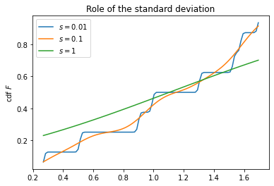
Can you characterize the graph of $F_{\text{kernel}}(z)$ if $s$ is close to $0$? Relatively large?
* Close to the empirical distribution function because the summands are closing to the theta-function, quickly varying from $0$ to $1$ in a small neighborhood of the existed values $x_i$ (because $s$ is small)* As $s$ increases the approximation becomes smoother because the range of the values characterizes the variation of each summand is wider
* Eventually this range becomes too wide, jumps at the observed values disappear, and the approximation is irrelevant
import numpy as np
a = 5.0
type(a) == int
#function returns cdf with the normal kernel defined above and the support on [min(x), max(x)]
#s = 0.3*np.std(x) / ((len(x))**0.2)

#error processing
#code generates pairs: value of random variable and cdf at this point
#values:
#   between min(x) and max(x) with a uniform step, where the equation is used
#   two additional values: one at the left, where cdf = 0, and one at the right, where cdf = 1
from scipy.stats import norm
def cdf_kernel_norm(x, s=None, num=100):
    func_name = 'cdf_kernel_norm' #for error messages
    #Error processing
    if s == None:
        s = 0.3*np.std(x) / ((len(x))**0.2)
    if type(num) != int:
        raise TypeError(f'{func_name}: Only integer <num> are allowed; transfered: {num}')
    elif num <= 0:
        raise Exception(f'{func_name}: incorrect number of variables <num> = {num}')
    if x == None or len(x) == 0:
        raise Exception(f'{func_name}: Incorrect input array {x}')
    #----End of error processing
    # The simplest way to define the values is z = np.linspace(min(x), max(x), num)
    # We define additionally min(x) - delta, where cdf = 0 and max(x) + delta, where cdf = 1
    # normally delta = x[i+1] - x[i], but a certain definition must be done if len(x) == 1
    elif len(x) == 1 and x != 0:
        delta = x[0] / 2
        z = np.array([x[0]-delta, x[0], x[0]+delta])#values at which cdf is defined
    elif len(x) == 1:
        delta = 1
        z = np.array([x[0]-delta, x[0], x[0]+delta])#values at which cdf is defined
    else:
        delta = (np.max(x) - np.min(x)) / (len(x) - 1)
        z = np.linspace(min(x)-delta, max(x)+delta, num+2)#values at which cdf is defined
    cdf = []
    cdf.append(0)
    for zz in z[1:-1]:
        arr = [norm.cdf((zz-xx) / s) for xx in x]
        cdf.append(np.mean(arr)) #the value of cdf at the point z
    cdf.append[1]
    return z, cdf
Role of the parameter $s$
- The next two cells highlight the role of the parameter $s$
- The parameters is naturally measured in standard deviations
- Possible (to some extent universal) choice is in the second cell
x = []
N = 8
random.seed(1)
for _ in range(N):
    x.append(random.uniform(0, 2))
x = np.array(sorted(x))

fig, ax = plt.subplots(1, 1)
s_param = [0.01, 0.1, 1]
for s in s_param:
    z, cdf = cdf_kernel_norm(x, s)
    plt.plot(z, cdf, label=f'$s = {s}$')
ax.set_ylabel('cdf $F$')
ax.set_title('Role of the standard deviation')
ax.legend()
plt.show()
fig, ax = plt.subplots(1, 1)
plt_empirical_dstr(x)
z, cdf = cdf_kernel_norm(x, s)#Kernel approximation
plt.plot(z, cdf)
ax.set_xlabel('observed values of the random variable')
ax.set_ylabel('cdf $F$')
ax.set_title('${:d}$-value sample'.format(N))
ax.legend()
plt.show()
from scipy.interpolate import interp1d
import random

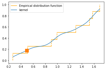
def plt_kernel_appr(x, s=None, numpoints=100, label='kernel'):
    if s == None:
        s = 0.3*np.std(x) / ((len(x))**0.2)
    z, cdf = cdf_kernel_norm(x, s)
    ppf_str = interp1d(cdf, z, kind='linear')
    tt = np.linspace(min(cdf), max(cdf), numpoints)
    ax.plot(ppf_str(tt), tt, label=label)

fig, ax = plt.subplots(1, 1)
plt_empirical_dstr(x)
random.seed(1)
v_tmp = random.uniform(min(cdf), max(cdf))
plt_kernel_appr(x)
ax.plot(ppf_str(v_tmp), v_tmp, 's', markersize=12)
ax.legend()
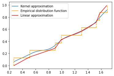
Comparison of percentile and kernel approximations
def cdf_percentile_appr(x, num_percentiles=100):
    t = []
    val = []
    for uni in range(num_percentiles):
        t.append(uni / num_percentiles)
        val.append(np.percentile(x, uni))
    return val, t

random.seed(1)
fig, ax = plt.subplots(1, 1)
plt_kernel_appr(x, label='Kernel approximation')
plt_empirical_dstr(x)
val, t = cdf_percentile_appr(x)
ax.plot(val, t, label='Linear approximation', color='red')
ax.legend()
plt.show()
Bootstrap and bias reduction
- $\hat{θ}$ is a consistent biased estimator. Target: to reduce the bias.
- Solution:
- Let $\theta$ be the true value; $\mathbf{x}$ be the initial sample. Then $\mathbf{E}\,\theta = \theta+b$
- Estimate the expected value with the bootstrap. Namely, repeat $N$ times:
- bootstrap a sample $\mathbf{x}^*$ from $\mathbf{x}$
- find estimate $\hat{\theta^*_i}$ with $\mathbf{x}^*$
- compute $\widehat{\mathbf{E}\,\theta} = \frac{1}{N} \sum_{i=1}^N \hat{\theta^*_i}$
- Use the equation $\widehat{\mathbf{E}\,\theta} = \hat{\theta} + \hat{b}$ to estimate the bias.
- Subtract the estimate of the bias from the estimate:
$\newcommand{\Exp}{\mathbf{E}\,}$
Bias reduction. Example
- $\mathbf{x} = x_1, \ldots, x_n$ is a sample from the uniform distribution $U(0, \theta)$
- Let's use the largest value $x_{(n)}$ as an estimate of $\theta$
Question: Prove that $\hat{\theta} = X_{(n)}$ is the MLE estimator
* Hint: $X_{(n)}- Bootstrap sample $\mathbf{x}^*$ from $\mathbf{x}$ of size $n$ and find $\max(\mathbf{x}^*)$
- Repeat $N$ times, find the average of the estimates and reduce the bias
#Example with $n = 15$, $N = 1000$, $\theta = 2$
import numpy as np
import random
random.seed(1)
n = 15
N = 1000
theta = 2
x = []
for _ in range(N):
    x.append(random.uniform(0, theta))
#data is sampled; theta is a secret knowledge
theta_mle = max(x)
thetas_bootstrap = []
for i in range(N):
    x_tmp = random.choices(x, k=len(x))
    thetas_bootstrap.append(np.max(x_tmp))
theta_corrected = 2*theta_mle - np.mean(thetas_bootstrap)
print('True value = {:.6f}; initial estimate = {:.6f}; corrected estimate = {:.6f}'.format(theta,
                                                                        theta_mle, theta_corrected))
Let $X_1$, $\ldots$, $X_n$ be distinct observations (no ties). Show that there are $2n-1\choose n$ distinct bootstrap samples. Note that this number is asymptotically $(n\pi)^{-1/2} 2^{2n-1}$
Summary
- Generation of the sample from given distribution. The problem is to create the inverse cdf
- Bootstrap
