General Concepts of Parameter Estimation
Overview
In this part of the tutorial, we address the problem of the parameter estimation. You may hypothesize that the observed data is drawn from a certain class of the distribution. For example, the data look like a known distribution, or the underlying mechanism can lead to the distribution of a certain type, or you try to distinguish between different types of the distribution. In all these cases, you should estimate unknown parameters of the distribution. The reported estimate consists of a value and the plus-minus component that indicates the uncertainty of the estimate. We'll consider standard methods discussing pro and contra.
MLE: Basic
- $\mathbf{x} = (x_1, \ldots, x_n)$ is the sample from (unknown) distribution
- $\theta$ is the parameter of the distribution, we want to estimate
- $\hat{\theta} = g(\mathbf{x}) = g(x_1, \ldots, x_n)$ is a function that is defined to estimate the unknown parameter
- The value $\hat{\theta}$ depends on the sample. The value $\hat{\theta} = g(\mathbf{x})$ found with a specific sample is called an estimate
- The estimate is expected to be close to the true value $\theta$
$\newcommand{\Prob}[1]{\mathsf{P}\{#1\}}$
$\newcommand{\Exp}{\mathbf{E}}$
As estimates depend on a sample they can be considered as random variables. One may say that each $x_i$ is the observation of an unknown distribution (random variable) $X_i$, where $X_i$ are independent and have a common probability density $f$. Then the expected value of $\hat{\theta}(\mathbf{X}) = g(X_1, \ldots, X_n)$ are defined as
$$ \Exp\big(\hat{\theta}(\mathbf{X})\big) = \int \hat{\theta}(\mathbf{x}) \underbrace{f(x_1) \ldots f(x_n)}_{\text{joint density}} \, d\mathbf{x} $$$$ \text{BIAS: } b = \Exp\big(\hat{\theta}(\mathbf{X})\big) - \theta \quad \text{Unbiased estimate: } b = 0 $$$\newcommand{\Exp}{\mathbf{E}}$ $\newcommand{\Var}{\mathbf{Var}}$
The mean square error is expanded into the sum of squares of statistical and systematic errors.
Prove
$\newcommand{\Exp}{\mathbf{E}}$ $\newcommand{\Var}{\mathbf{Var}}$
is an unbiased estimator for the covariance $V_{xy}$ of two random variables $x$ and $y$
$\newcommand{\Exp}{\mathbf{E}}$ $\newcommand{\Var}{\mathbf{Var}}$
Definition $$ \Var\,\hat{\theta} = \Exp(\hat{\theta}^2) - \big(\Exp\hat{\theta}\big)^2 $$
where $\mu_k$ is the $k$th central moment
Maximum likelihood
$\newcommand{\Prob}[1]{\mathsf{P}\{#1\}}$
- \eqref{e:mle:goal} measures the probability to observe the sample under assumption that it is generated from the distribution $f(x;\theta)$
- In this equation, $dx_i$ are fixed as small predefined constants, $x_i$ are fixed as given values of the sample
- A single unknown is $\theta$, which is chosen to maximize the probability \eqref{e:mle:goal}
More practical, to maximize the log-likelihood function $$ \log L(\theta) = \sum_i \log(f(x_i;\theta)) \to max $$ Equalizing derivative to zero $$ \sum_i \frac{f'_{\theta}(x_i;\theta)}{f(x_i;\theta)} = 0 $$ $\hat{\theta}$ solves the above equation
Equalizing the derivative to zero: $$ -\frac{n}{\tau} + \sum_i \frac{t_i}{\tau^2} = 0 \quad\text{or}\quad \hat{\tau} = \bar{t} $$
populate the cell with the following code to generate 100 values from the uniform random variable on $[0, 1]$
import numpy as np
from scipy.stats import expon
import matplotlib.pyplot as plt
import random
def expon_sample(a=1, num=1):
    z = np.array([random.uniform(0, 1) for _ in range(num)]) #generate num random numbers between 0 and 1
    x = expon.ppf(z)/a
    return x
x = expon_sample(num=100)
The library alternative (for $a=1$) is
t = expon.rvs(size=100)
import numpy as np
from scipy.stats import expon
import matplotlib.pyplot as plt
import random
random.seed(1)
#generation of <num> values from the exponential random variable with the parameter a
#default: a = 1, num = 1
def expon_sample(a=1, num=1):
    z = np.array([random.uniform(0, 1) for _ in range(num)]) #generate num random numbers between 0 and 1
    x = expon.ppf(z)/a
    return x
t = expon_sample(num=100)
- We are ready to solve numerically the following problem.
- The sample $t$ is generated from the exponential distribution with the unknown mean $\tau$. What is the estimates of $\tau$?
- Applying $\hat{\tau} = \bar{t}$, we get
tau_est = np.mean(t)
tau_est
Question:
$\hat{\theta}$ is the MLE estimator of $\theta$. What is the MLE estimator for $h(\theta)$?
* $\displaystyle\frac{\partial L}{\partial \theta} =
\frac{\partial L}{\partial h}
\frac{\partial h}{\partial \theta} $
* If $h'_{\theta} \ne 0$, then $h(\hat{\theta})$ is the MLE estimator for $\widehat{h(\theta)}$
$\newcommand{\Exp}{\mathbf{E}}$
Example: Estimation of the decay $1/\tau$ of the exponential distribution
- $\hat{\lambda} = \frac{1}{\bar{t}}$ is the MLE estimator of the decay $\lambda = 1/\tau$ of the exponential distribution
- However, by Jensen's inequality $\varphi(\Exp X) \le \Exp\varphi(X)$ for any convex function $\varphi$:
$$
$$\frac{1}{\Exp X} \le \Exp\left(\frac{1}{X}\right), \quad \Exp\hat{\lambda} = \Exp(1/\hat{\tau}) \ge 1 / \Exp\tau
Example: Normal distribution $\mathbf{N}(\mu, \sigma^2)$
Variance of MLE
Example: Exponential distribution: expected value
$\newcommand{\Var}{\mathbf{Var}}$ $$ \Var\,\hat{\tau} = \Var\left( \frac{X_1 + \ldots + X_n}{n} \right) = \frac{\sigma^2}{n} = \frac{\tau^2}{n} $$ Then if the estimate $\hat{\tau} = 1.011$ is obtained with the sample of the size $100$ (as above) then the standard deviation of the estimate is $1.011 / \sqrt{100} = 0.1011$. The reported record may be $\hat{\tau} = 1.011 \pm 0.101$. In this example, the estimate of the parameter is substituted for the unknown value of the parameter; $\hat{\tau}$ is used instead of $\tau$ in the last equation
- Monte-Carlo method: simulate a large number of experiments
- compute MLE each time and construct the distribution of MLE
- The mean and the standard deviation of the MLE distribution is used to indicate the parameter value and the plus/minus component
- Asymptotic normality of MLE is frequently observed
Example: Return to the exponential distribution
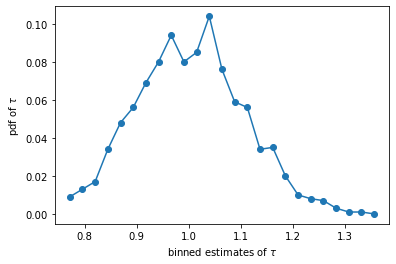
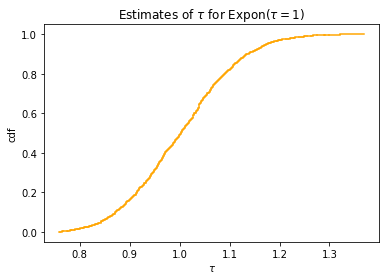
- compute the distribution of the estimated expected value
- repeat the construction of the sample and the estimate of the expected value $N = 1000$ times
N = 1000
tau_val = np.sort([np.mean(expon_sample(num=100)) for _ in range(N)])
The following cells are technical. They display the "histogram" and the empirical distribution function
#Empirical probability density function
import math

def pdf_my(array, n_bins = 10, arr_min = [], arr_max = []):
    array = np.array(array)
    if np.size(arr_min) == 0:
        arr_min = np.min(array)
    if np.size(arr_max) == 0:
        arr_max = np.max(array)
    if n_bins == 0:
        raise Exception('At least 1 bin required')
    else:
        x = []
        y = []
        gap = (arr_max - arr_min) / n_bins
        for i in range(n_bins):
            x.append(arr_min + (0.5 + i) * gap)
            y.append(0)
        n_els = 0
        for arr in array:
            cur = int(math.floor((arr - arr_min) / gap))
            if cur >= 0 and cur < n_bins:
                y[cur] += 1
                n_els += 1
        if n_els > 0:
            for cur in range(len(y)):
                y[cur] = y[cur] / n_els
    return x, y
np.size(tau_val)
fix, ax = plt.subplots(1, 1)
tau, y = pdf_my(tau_val, 25)
ax.plot(tau, y, marker = 'o')
ax.set_xlabel(r'binned estimates of $\tau$')
ax.set_ylabel(r'pdf of $\tau$')
#technical: plots empirical distribution (step-like function)
def plt_empirical_dstr(x, clr='orange', label='Empirical distribution function'):
    frac_before = [i / len(x) for i in range(len(x))]
    frac_after = [(i+1) / len(x) for i in range(len(x))]
    for i in range(len(x)):
        plt.plot([x[i], x[i]], [frac_before[i], frac_after[i]], linestyle='--',
                color=clr)
        if i == 0:
            plt.plot([x[i], x[i+1]], [frac_after[i], frac_after[i]], label=label,
                    color=clr)
        elif i < len(x)-1:
            plt.plot([x[i], x[i+1]], [frac_after[i], frac_after[i]],
                    color=clr)
plt_empirical_dstr(tau_val)
plt.xlabel('$\\tau$')
plt.ylabel('cdf')
plt.title('Estimates of $\\tau$ for Expon($\\tau=1$)')
the variance of the estimate is the variance of the sample of estimates:
est_var = np.var(tau_val)
est_std = np.std(tau_val)
est_var, est_std
The initial estimate can be taken as the center of the interval
print('Estimate of the expected value: {:.3f}\u00B1{:.3f}'.format(tau_est, est_std))
However with several experiments, the mean of the estimates is a better candidate
print('Estimate of the expected value: {:.4f}\u00B1{:.4f}'.format(np.mean(tau_val), est_std))
Rao-Cramer Inequality and Fisher Information
$\newcommand{\Exp}{\mathbf{E}}$ $\newcommand{\Var}{\mathbf{Var}}$
The Rao-Cramer inequality reads that $$ \Var(\hat{\theta}^*) \ge \frac{\left(1+\frac{\partial \mathbf{b}(\hat{\theta})}{\partial \theta}\right)^2} {\Exp\left( -\frac{\partial^2 l_n}{\partial \theta^2} \right)}, $$ where $\mathbf{b}$ is the bias of the estimate $\hat{\theta}$, $l_n(\mathbf{x})$ is the likelihood function, given unknown $\theta$, and the expected value is computed with respect to the probability density $f(\mathbf{x}|\theta)$.
The denominator in the Rao-Cramer inequality is called the Fisher information derived from the sample. If a single observation of the distribution with the density $f(x|\theta)$ is performed than the Fisher information is given by the equation
$$ \mathbf{I} = \int_{-\infty}^{+\infty} -\frac{\partial^2 \log(f(x|\theta))}{\partial \theta^2} f(x|\theta) \, dx $$Example of statistics to quantify the correspondence
- If $n_{\text{tot}}$ is treated as the Poisson random with the mean $\nu_{\text{tot}}$, and
- The likelihood ratio is
where ${\nu}$ is changed to its estimates $\hat{{\nu}}$.
- The statistics
follows a $\chi^2$ distribution with $N-m$ degrees of freedom, where $m$ is the number of parameters estimated from the data ($m=1$ if just the expected value of the exponential distribution is estimated).
- The terms with $n_i = 0$ are excluded as $n_i^{n_i}\to 1$ as $n_i \to 0$, and the corresponding terms are equal to $1$ in the product defining $\lambda$
- The quantity $\displaystyle\lambda(\nu) = \frac{L(\mathbf{n}|{\nu})}{L(\mathbf{n}|\mathbf{n})}$ only differs from the likelihood function by the factor $L(n|n)$, which does not depend on the parameters
- The parameters that maximize $\lambda(\nu)$ are therefore equal to the MLE; $\lambda({\nu})$ can be used both for constructing estimators as well as for testing goodness-of-fit
As we discussed earlier, the Pearson test is applicable to the binned data. To recall:
- $n_{\text{tot}}$ is treated as a Poisson random variable
- $n_{\text{tot}}$ is fixed
$m$ is the number of estimated parameters
For finite data samples, none of the statistics given above follow exactly the $\chi^2$ distribution. If the histogram contains bins with, for example, $n_i < 5$, a Monte Carlo study can be carried out to determine the true $\texttt{pdf}$, which can then be used to obtain a $p$-value.
- two-sided alternatives: $H_1$: $\theta\ne\theta_0$
- The log-likelihood under $H_1$ is unrestricted maximum
- Let $\hat{\theta}$ be the MLE of $\theta$. Then the logarithm of the likelihood ratio is $l_n(\hat{\theta})-l_n(\theta_0)$. The test rejects $\theta_0$ if $t = l_n(\hat{\theta})-l_n(\theta_0) > c$, where $c$ is determined through the standard condition $\Prob{t > c \,|\, \theta_0} = \alpha$.
MLE and Bayesian estimators
With ML, we focus on the conditional probability density function for $\theta$ given the probability density of data: $P(\theta|x)$. This is obtained from the likelihood via Bayes' theorem: $$ p(\theta | x) = \frac{L(x|\theta)\Prob{\theta}}{\int L(x|\theta')\Prob{\theta'} d\theta'} $$ Here $\Prob{\theta}$ is the prior probability density for $\theta$, reflecting the state of knowledge of $\theta$ before the consideration of the data, and $p(\theta|x)$ is called the posterior probability density for $\theta$ given the data $x$.
In Bayesian statistics, all our knowledge about $\theta$ is contained in $p(\theta|x)$. Since it is rarely practical to report the entire probability distribution function, an appropriate way of summarizing it must be found. The first step in this direction is an estimator, which is often taken to be the value of $\theta$ at which $p(\theta|x)$ is a maximum. If the prior probability distribution function $\Prob{\theta}$ is taken to be a constant, then $p(\theta|x)$ is proportional to the likelihood function $L(x|\theta)$, and the Bayesian and ML estimators coincide. The ML estimator can be regarded as a special case of a Bayesian estimator, based on a uniform prior probability distribution function.
Question:
Is it correct that the Bayesian estimator is a special case of the ML estimator?
Is it correct that the ML estimator is a special case of the Bayesian estimator?
* No
* Yes; if the prior probabilities are the same
Method of Moments
- When MLE are difficult to compute equalize
- $\displaystyle \frac{1}{n} \sum_{i=1}^n x_i^k = \int x^k f(x;{\theta}) \, dx, $, $k=1,\ldots,N$,
and the number of unknown parameters is also $N$: ${\theta} = (\theta_1,\ldots,\theta_N)$ - The solution of the algebraic system of the equations gives the estimates $\hat{{\theta}}$ of ${\theta}$
Confidence intervals
- If the limit distribution of the unknown parameter is Gaussian, then the standard deviation of the estimates exhibits the uncertainty of measurement and can be referred to as the standard error
- The computation is based on, f.~e., theoretical reasoning or Monte-Carlo / bootstrap methods
- We turn to the case characterized by non-Gaussian limit behavior of the estimated parameter
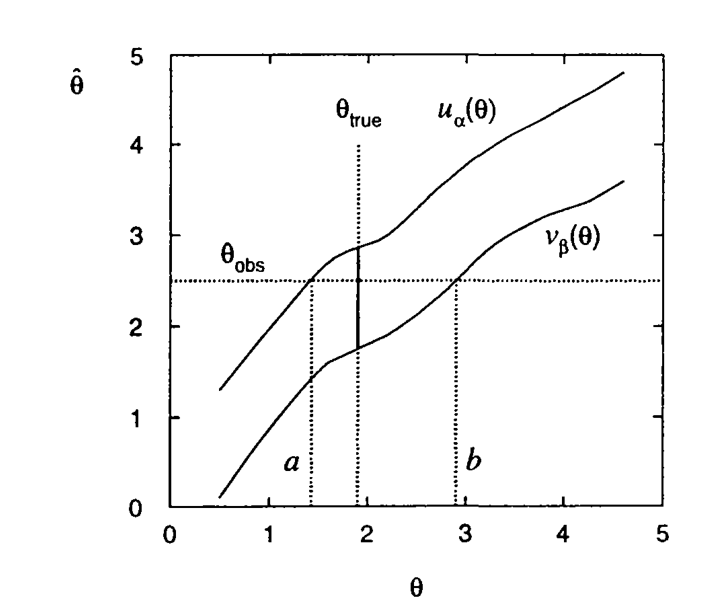
- $\hat{\theta}(x_1,\ldots,x_n)$ is an estimator for a parameter $\theta$ based on the sample $\mathbf{x}$
- The distribution $g(\hat{\theta};\theta) = G'(\hat{\theta};\theta)$ is known through the analytical determination or a Monte Carlo computation. Warning: the true value of $\theta$ is not known, but the distribution $g$ is known (estimated) for any given value of $\theta$.
- Introduce a lower $\beta$ and upper $\alpha$ quantiles of the distribution \begin{gather*} \alpha = \Prob{\hat{\theta} \ge u_{\alpha(\theta)}} = 1 - G(u_{\alpha}(\theta); \theta), \\ \beta = \Prob{\hat{\theta} \le v_{\beta(\theta)}} = G(v_{\beta}(\theta); \theta), \end{gather*}
# Step-like empirical distribution function (continious at the right)
freq_before = [i / N for i in range(N)]
Example of a code that creates the pdf from cdf
from plt_fit import regress
def smooth(x, y, num_smooth=100):
    x_new = []
    slp = []
    delta = (np.max(x) - np.min(x)) / len(x)
    for i in range(num_smooth-1):
        wnd_x = []
        wnd_y = []
        for j in range(num_smooth):
            if j < num_smooth-i:
                wnd_x.append(x[0] - (num_smooth-i-j)*delta)
                wnd_y.append(0)
            else:
                wnd_x.append(x[j-(num_smooth-i)])
                wnd_y.append(y[j-(num_smooth-i)])
        slope, intercept, xfit1, yfit1 = regress(np.array(wnd_x), np.array(wnd_y))
        x_new.append(np.mean(x[0:i+1]))
        slp.append(slope)
    for i in range(len(y)-num_smooth+1):
        x_new.append(np.mean(x[i:i+num_smooth-1]))
        slope, intercept, xfit1, yfit1 = regress(np.array(x[i:i+num_smooth-1]),
                                             np.array(y[i:i+num_smooth-1]))
        slp.append(slope)
    for i in range(num_smooth-1):
        wnd_x = list(x[len(x)-num_smooth+i:len(x)])
        wnd_y = list(y[len(x)-num_smooth+i:len(x)])
        for j in range(len(wnd_x), num_smooth):
            wnd_x.append(x[-1] + (j-len(wnd_x)+1)*delta)
            wnd_y.append(1)
        slope, intercept, xfit1, yfit1 = regress(np.array(wnd_x), np.array(wnd_y))
        x_new.append(np.mean(x[len(x)-num_smooth+i:len(x)]))
        slp.append(slope)
    x_new.append(x[-1])
    slp.append(0)
    return x_new, slp
fig, ax = plt.subplots(1, 1)
x_new, slp = smooth(tau_val, freq_before, num_smooth=100)
plt.plot(x_new, slp)
plt.title('Approximation to the empirical density of the $\\tau$-estimates')
Computation of the $\alpha$ and $\beta$ quantiles based on the cdf
alpha = 0.005
beta = 0.005
#for the sake of simplicity, avoid the interpolation
i_left = int(alpha*N)
i_rght = int((1-beta)*N)
t_left = tau_val[i_left]
t_rght = tau_val[i_rght]
print(t_left, t_rght)
- $\hat{\theta}(x_1,\ldots,x_n)$ is an estimator for a parameter $\theta$ based on the sample $\mathbf{x}$
- The distribution $g(\hat{\theta};\theta) = G'(\hat{\theta};\theta)$ is known through the analytical determination or a Monte Carlo computation. Warning: the true value of $\theta$ is \emph{not} known, but the distribution $g$ is known (estimated) for any given value of $\theta$.
- Introduce a lower $\beta$ and upper $\alpha$ quantiles of the distribution \begin{gather*} \alpha = \Prob{\hat{\theta} \ge u_{\alpha(\theta)}} = 1 - G(u_{\alpha}(\theta); \theta), \\ \beta = \Prob{\hat{\theta} \le v_{\beta(\theta)}} = 1 - G(u_{\alpha}(\theta); \theta), \end{gather*}
 |
- As long as $u_{\alpha}(\theta)$ and $v_{\beta}(\theta)$ are monotonically increasing functions of $\theta$ (a general case), the inverse function are well defined:
- Then
and $$ \Prob{a(\hat{\theta}) \le {\theta} \le b(\hat{\theta})} = 1 - \alpha - \beta $$
- $[a,b]$ is called confidence interval at a confidence level of $1-\alpha-\beta$
Question:
You estimated the parameter $\tau$ of the exponential distribution $F(t) = 1-e^{-t/\tau}$, $t>0$, with the estimates $\hat{\tau} = \bar{\mathbf{x}}$, where $\mathbf{x} = (x_1, \ldots, x_n)$ denotes $n=20$ independent observations. You found that $[0.95,1.07]$ is the symmetrical confidence interval for the estimate $\hat{\tau}$ at the confidence level $0.99$ What is the $0.99$ symmetric confidence interval for the unknown parameter $\tau$?
* Hint: recall the distribution of the sum of independent exponential random variables $X_1 + \ldots + X_n$
Special important case: the distribution of $\hat{\theta}$ is Gaussian with the mean $\theta$ and the standard deviation $\sigma$. Then the cdf is \begin{equation} G(\hat{\theta}; \theta, \sigma) = \int_{-\infty}^{\hat{\theta}} \frac{1}{\sqrt{2\pi \sigma^2}} e^{\frac{-(\hat{\theta}' - \theta)^2}{2\sigma^2}}\, d\hat{\theta}' \label{e:confidence:gauscdf} \end{equation} This case is general because any estimator that is a linear function of a sum of random variables becomes Gaussian in the large sample limit, according to the central limit theorem. Assumption (\ref{e:confidence:gauscdf}) simplifies the construction of the confidence interval.
If $\sigma$ is known, the boundaries of the confidence interval are given by the equations $$ \alpha = 1 - G(\hat{\theta}; a, \sigma) = 1 - \Phi\left( \frac{\hat{\theta}-a}{\sigma} \right) $$ $$ \beta = G(\hat{\theta}; b, \sigma) = \Phi\left( \frac{\hat{\theta}-b}{\sigma} \right) $$ Eventually, $$ a = \hat{\theta} - \sigma\Phi^{-1}(1-\alpha), \quad b = \hat{\theta} - \sigma\Phi^{-1}(\beta) = \hat{\theta} + \sigma\Phi^{-1}(1-\beta), $$
- $\sigma$ as a plus/minus component was used earlier; it corresponds to the $0.68$ confidence interval
- $[\hat{\theta} - 2\sigma, \hat{\theta} + 2\sigma]$ is the $0.96$ confidence interval
- If the standard deviation $\sigma$ is not known:
- the volume $n$ of the sample is large, apply the confidence interval based on the Gaussian distribution
- Otherwise, relate the cumulative distribution $G(\hat{\theta}; \theta, \sigma)$ to Student's $t$-distribution (Dudewicz & Mishra, Modern Mathematical Statistics, John WileY, 1988; section 10.2)
- If the distribution of the estimate is not Gaussian or not known analytically, sometimes there is a transformation $\theta \to \varphi(\theta)$ such that the new variable is approximately Gaussian
Question:
Return to the estimate of the parameter $\tau$ of the exponential distribution $F(t) = 1-e^{-t/\tau}$, $t>0$, with the estimates $\hat{\tau} = \bar{\mathbf{x}}$, where $\mathbf{x} = (x_1, \ldots, x_n)$ denotes $n=20$ independent observations and $[0.95,1.07]$ is the $0.99$ symmetrical confidence interval for the estimate. If you use the normal approximation with $\sigma = \sqrt{0.5\cdot(0.95+1.07)}$, what is the $0.99$ symmetric confidence interval for the unknown parameter $\tau$?
We discussed
- the estimate of the maximum likelihood addressing the questions of the likelihood function, log-likelihood function and its maximization
- the estimates obtained with the method of moments
- uncertainty of the estimates based on
- its variance computed with
- the true distribution
- Monte-Carlo simulations
- asymptotic distribution
- Rao-Cramer lower bound of the estimate
- confidence interval
- its variance computed with

